Introducing the K-D-trees data structure – Arrays, collections and data structures
114. Introducing the K-D-trees data structure
A K-D Tree (also referred to as a K-Dimensional tree) is a data structure that is a flavor of Binary Search Tree (BST) dedicated to holding and organizing points/coordinates in a K-dimensional space (2-D, 3-D, and so on). Each node of a K-D Tree holds a point representing a multi-dimensional space. The following snippet shapes a node of a 2-D Tree:
private final class Node {
private final double[] coords;
private Node left;
private Node right;
public Node(double[] coords) {
this.coords = coords;
}
…
}
Instead of a double[] array you may prefer java.awt.geom.Point2D that is dedicated to represent a location in (x, y) coordinate space.Commonly, K-D Trees are useful for performing different kinds of searches such as nearest neighbor searches and range queries. For instance, let’s assume a 2-D space and a bunch of (x, y) coordinates in this space:
double[][] coords = {
{3, 5}, {1, 4}, {5, 4}, {2, 3}, {4, 2}, {3, 2},
{5, 2}, {2, 1}, {2, 4}, {2, 5}
};
We can represent these coordinates as we commonly know in an X-Y coordinates system, but we can also store them in a K-2D Tree as in the following figure:
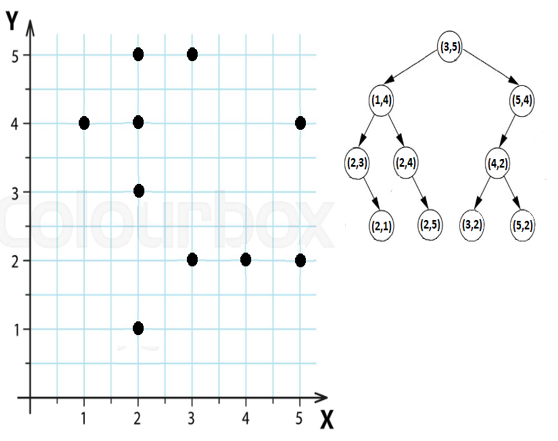
Figure 5.20 – A 2D space represented in X-Y coordinates system and K-2D Tree
But, how did we build the K-D Tree?
Inserting in a K-D Tree
We insert our coordinates (cords) one by one starting with coords[0] = (3, 5). The (3, 5) pair becomes the root of the K-D Tree. The next pair of coordinates is (1, 4). We compare x of the root with x of this pair and we notice that 1 < 3 which means that (1, 4) goes as the left child of the root. The next pair is (5, 4). At the first level, we compare the x of the root with 5 and we have that 5 > 3, so (5, 4) goes as the right child of the root. The following figure reveals the insertion of (3, 5), (1, 4), and (5, 4).
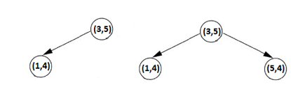
Figure 5.21 – Inserting (3, 5), (1, 4), and (5, 4)
Next, we insert the pair (2, 3). We compare the x components of (2, 3) and (3, 5) and we have that 2 < 3, so (2, 3) goes to the left of the root. Next, we compare the y component of (2, 3) and (1, 4) and we have that 3 < 4 so (2, 3) goes to the left of (1, 4).Next, we insert the pair (4, 2). We compare the x components of (4, 2) and (3, 5) and we have that 4 > 3, so (4, 2) goes to the right of the root. Next, we compare the y component of (4, 2) and (5, 4) and we have that 2 < 4 so (4, 2) goes to the left of (5, 4). The following figure reveals the insertion of (2, 3), and (4, 2).
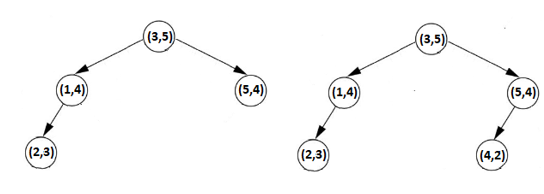
Figure 5.22 – Inserting (2, 3) and (4, 2)
Next, we insert the pair (3, 2). We compare the x components of (3, 2) and (3, 5) and we have that 3 = 3, so (3, 2) goes to the right of the root. Next, we compare the y component of (3, 2) and (5, 4) and we have that 2 < 4 so (3, 2) goes to the left of (5, 4). Next, we compare the x component of (3, 2) and (4, 2) and we have that 3 < 4 so (3, 2) goes to the left of (4, 2).Next, we insert the pair (5, 2). We compare the x components of (5, 2) and (3, 5) and we have that 5 > 3, so (5, 2) goes to the right of the root. Next, we compare the y component of (5, 2) and (5, 4) and we have that 2 < 4 so (5, 2) goes to the left of (5, 4). Next, we compare the x component of (5, 2) and (4, 2) and we have that 5 > 4 so (5, 2) goes to the right of (4, 2). The following figure reveals the insertion of (3, 2) , and (5, 2).
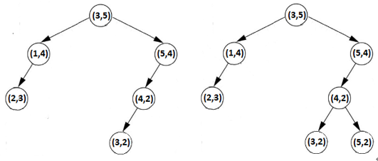
Figure 2.23 – Inserting (3, 2) and (5, 2)
Next, we insert the pair (2, 1). We compare the x components of (2, 1) and (3, 5) and we have that 2 < 3, so (2, 1) goes to the left of the root. Next, we compare the y component of (2, 1) and (1, 4) and we have that 1 < 4 so (2, 1) goes to the left of (1, 4). Next, we compare the x component of (2, 1) and (2, 3) and we have that 2 = 2 so (2, 1) goes to the right of (2, 3).Next, we insert the pair (2, 4). We compare the x components of (2, 4) and (3, 5) and we have that 2 < 3, so (2, 4) goes to the left of the root. Next, we compare the y component of (2, 4) and (1, 4) and we have that 4 = 4 so (2, 4) goes to the right of (1, 4).Finally, we insert the pair (2, 5). We compare the x components of (2, 5) and (3, 5) and we have that 2 < 3, so (2, 5) goes to the left of the root. Next, we compare the y component of (2, 5) and (1, 4) and we have that 5 > 4 so (2, 5) goes to the right of (1, 4). Next, we compare the x component of (2, 5) and (2, 4) and we have that 2 = 2 so (2, 5) goes to the right of (2, 4). The following figure reveals the insertion of (2, 1) , (2, 4), and (2, 5).
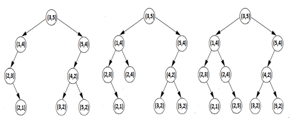
Figure 2.24 – Inserting (2, 1), (2, 4), and (2, 5)